Basic Upper Air Analysis

Upper level charts for 00 UTC Nov. 10, 1998, showing geopotential height (black contours), temperature (red contours), and observed winds. Contour interval 30 m for 850- and 700-hPa height, 60 m for 150-hPa height, 120 m for 250- and 200-hPa, and 60 m for 100-hPa height. The contour interval for temperature is 4 degrees celsius in the left panels and 2 degrees celsius in the right panels. The shading in the 250-hPa chart are isotachs defining the position of the jet stream. [Wallace and Hobbs 329]

Synoptic charts at 00, 09, and 18 UTC Nov 10, 1998. (Left) The 500-hPa height (contours at 60-m intervals; labels in dkm) and relative vorticity (blue shading; scale on color bar in units of 10^(-4) s^(-1)). (Right) Sea-level pressure (contours at 4-hPa intervals) and 1000- to 500-hPa thickness (colored shading: contour interval 60-m; labels in dkm). Surface frontal positions, as defined by a skilled human analyst, are overlaid. [Wallace and Hobbs 315]

1000-500 mb / SLP Chart

• Includes SLP and 1000-500 mb thickness
• Given distribution of geopotential height on any two pressure surfaces we can determine the distribution of thickness for the intervening layer.
• The "thickness" chart reveals temperature advection through the lower half of the troposphere.
• Frontal location: A cold front is usually placed at the leading edge of the greatest thickness packing (cold air advection) and a warm front is placed at the trailing edge (warm air advection
• 540 line: meaning 5400 meters between the 1000mb and the 500mb level.
• Often used to delineate the rain/snow line with snow expected on the cold side of that line and rain on the warm side (this is a rule of thumb, not a hard fast law)

800-mb Chart (~1,500 m)

• The 850-mb pressure surface is closest to the surface Through examination some differences should be mentioned:
• Solid lines are height contours (gpm).
• Dashed lines are isotherms (ºC).
• Closed lows at surface may appear as troughs @ 850 (in this case the winds stronger than at surface why? Less friction.
• Winds generally more parallel to height contours.
• Tilt of the cold front westward (backward) into the cold air as one goes up from the surface.
• Warm front is more clearly defined and farther poleward at 850.

[Wallace and Hobbs 329]

• Warm Air Advection
• Typically the greatest dynamically caused lifting mechanism over the large scale.
• Related to QG Theory.
• To be detailed in Synoptic Meteorology.

http://atsc.uga.edu/wx/ncep_loops.htm

700-mb Chart (3,000 m)

• Typically, the trough associated with surface lows are more difficult to identify and are displaced upstream (in this exceptional case, the low is still closed at 700 mb!)
• Further increase in wind speed
• Cold front located even farther west
• Warm front located much farther poleward and coincides with the location of the precipitation reaching ground.
• Frontal zones less clearly defined than at lower levels. (often difficult to detect equator-ward end of cold front).

[Wallace and Hobbs 329]

500-mb Chart (~5,000 m)

• Further upstream displacement of troughs.
• Strengthening of winds.
• Sloping of the frontal zones toward the cold air.
• Frontal zones hard to detect but thermal contrasts exist.

[Wallace and Hobbs 329]

250-mb Chart (~10,366 m)

• Near the climatological position of the polar jet stream.
• Warmest air (-44ºC) located north of jet stream near the  trough (over 4-Corners).
• Little to no advection as you go south.

[Wallace and Hobbs 329]

100-mb Chart (~16,000 m)

• Located well above the tropopause and jet stream.
• In stratosphere there is a marked decrease in wind speed when compared to 250-mb.
• Only planetary scale features present at 100 mb (not the synoptic scale).
• Temperature field reverses -- colder air as one goes toward the equator, warmer towards the poles.

[Wallace and Hobbs 329]

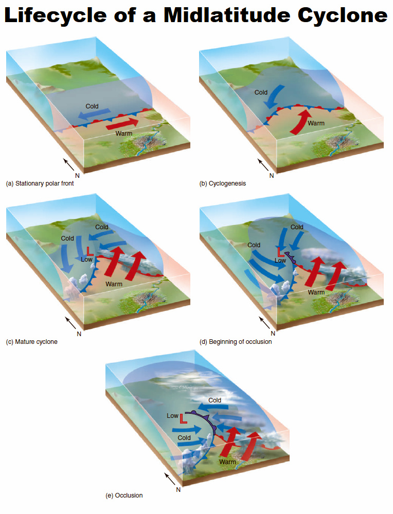
Three-Stage Model

• The three-stage model of an idealized mid-latitude (N.H.) cyclone with 1000-mb heights, 500-mb heights and 1000-500 mb thicknesses shows the development of the cyclone.
• Early Stage - surface low just beginning to form as wave along front on the warm side of the region of strong thickness contrast.
• Mature Stage - cold air starts streaming southward behind the surface low pressure area and warm air advances northward in advance of the cyclone.
• These distortions in the temp. field are reflected in the growing amplitude of the wave in the thickness pattern.The thickness pattern is closely related to the position of the warm and cold fronts.
• Surface low is in the process of passing under the jet stream, from the warm to cold side.
• Late Stage - the occlusion process has begun:
• The surface low moves across the thickness contours towards lower values as it deepens progressively farther back into the cold air.
• Junction of the warm and cold fronts remains on the warm side of the region of strong thickness contrast
• Occluded front coincides with a warm ridge in the thickness field.
• As the disturbance continues to amplify, the positions of the surface low and the 500-mb trough (or closed low) gradually begin to come into vertical alignment (stacked).
• In fully developed systems the vertical tilt completely disappears and all three sets of contours become mutually parallel.

(Top) Fields of 500-hPa height (thick black contours), 1000-hPa height (thin black contours), and 1000- to 500-hPa thickness (dashed red) at 00, 09, and 18 UTC Nov 10, 1998; contour interval 60-m for all three fields. Arrows indicate the sense of the geostrophic wind. (Bottom) Idealized depictions for a baroclinic wave and its attendant tropical extratropical cyclone its early (left), developing (center), and mature (right) stages. [Wallace and Hobbs 317]

Vertical Soundings

• Vertical soundings (found through radiosondes) show how the temp changes vertically with height, generally up to 100-mb or so.
• Backing -- counterclockwise winds; CAA.
• Veering -- clockwise winds; WAA.

Soundings of wind, temperature (red lines), and dew point (green lines) at 00 UTC Nov. 10, 1998 at Amarillo, Texas (left) in the cold frontal zone and Davenport, Iowa (right) in the warm frontal zone. [Wallace and Hobbs 331]

Sea-level pressure, surface winds, and frontal positions at 00, 09, and 18 UTC Nov. 10, 1998. Frontal symbols and wind symbols are plotted. The dashed blue line denotes the secondary cold front. The frontal positions are defined by a human analyst. [Wallace and Hobbs 319]

Vertical Cross Sections

• It is important to know the vertical structure of the atmosphere near a cold front.
• The forthcoming cross section was constructed using temps and wind soundings at locations between Riverton, WY, and Lake Charles, LA.
• Temps in ºC are solid red lines.
• Solid blue lines are isotachs (lines of constant wind speed) for the wind component normal to the section (positive into the section, negative out of the section).
• The section is oriented normal to the front and to the jet stream.

[Wallace and Hobbs 329]

Locations of the stations and vertical cross sections shown in this section. From north to south, KMQT is the station identifier for Marquette, Michigan; KRIW for Riverton, Wyoming; KLBF for North Platte, Nebraska; KSUX for Sioux Falls, South Dakota; KGAG for Gage, Oklahoma; KSGF for Springfield, Missouri; KBWG for Bowling Green, Kentucky; KCAE for Columbia, South Carolina; KJAN for Jackson, Mississippi; and KLCH for Lake Charles, Louisiana. [Wallace and Hobbs 339]

Screen capture from a PDF version of a powerpoint. Images from Wallace and Hobbs 319, 333, and 339.

Characteristics of Cross Section

• Well defined frontal zone in the lower troposphere, sloping toward the cold air with increasing height.
• Within the frontal zone the isotachs are sloping and very close together, wind component into the section is increasing very rapidly with height. This represents an area of strong vertical wind shear.
• Middle-latitude tropospheric jet stream is located within the gap in the tropopause where winds are the greatest (80 m/s)
• Reversal in the horizontal temp gradient between troposphere and stratosphere.

Isentropic Analysis

• Sometimes we use potential temp rather than temp in these cross section analysis.  We like isentropic analysis because:
• Under adiabatic conditions the isentropes in sections can be closely identified with air motion.
• In the figure the stability stratification is directly related to the vertical spacing of the isentropes.
• Regions of close spacing (i.e. the stratosphere and frontal zone) are characterized by strong static stability.

http://www-das.uwyo.edu/~geerts/cwx/notes/chap12/pot_vort.html

Screen capture from a PDF version of a powerpoint. Images from Wallace and Hobbs 319, 333, and 339.

Upper-Level Structure

• Understanding how cyclonic disturbances change over time requires a keen understanding of cyclones at various heights within the entire troposphere.
• Often we think of 500-mb winds as steering winds for features at the surface.
• The upper level patterns also act to influence the rates of intensification and weakening of surface cyclones and anticyclones, as well as the amounts of precip. associated with them.

Convergence and Divergence in a Column

• Convergence (divergence) within an air column is associated with increasing (decreasing) surface pressure, since the weight of the air column will increase (decrease) with time.
• Vertical motions in the atmosphere are related to divergence and convergence fields.

The relationship between divergence, convergence, and vertical motions in air columns. Black portions of arrows are outside the columns, while gray portions are inside. [Robert et al. 139]

Works Cited

Rauber, Robert M., et al. Severe and Hazardous Weather: An Introduction to High Impact Meteorology. 4th ed., Kendall Hunt, 2014.

Wallace, John, and Peter Hobbs. Atmospheric Science: An Introductory Survey. 2nd ed., Academic Press, 2006.

Extratropical / Midlatitude Cyclones

• Cyclone = any circulation around low-pressure.

• Extratropical Cyclone = large low-pressure system that often form in the mid-latitudes.

• Day-to-day weather in the mid- and high-latitudes is closely related to the location, development, and movement of cyclonic storms.

• Cyclones are responsible for:
• Changing air masses (temperature, dew point, wind, etc)
• Bringing precipitation opportunities

• Most weather is linked to extratropical cyclones, rather than being discrete weather events.

• Vertically speaking, they're found in the tropopause.

• Needed to balance temperature differences between the poles and equator (between the cold upper troposphere and the warm lower troposphere).

• Most intense in the late fall, winter and spring due to the temperature gradient between the tropics and the north pole being the strongest during that time.

• Winds blow counterclockwise (cyclonically) in the northern hemisphere and clockwise (cyclonically) in the southern hemisphere.

• It forms at intersecting fronts:
• Cold front is typically south and west, to east of the low.
• Cold air is "behind" the low, while warm air is "ahead" (lows and highs both move in the direction of the jet stream winds).
• Thunderstorms are often ahead of the cold front.
• Steady precipitation is often ahead of the warm front.

• Cloud Sequence: cirrus, cirrostratus, altostratus, nimbostratus

Norwegian / Bergen Cyclone Model

• During WWI, Vilhelm Bjerknes identified that midlatitude cyclones formed along the boundary separating polar air from the warmer air to the south.

• Widely used by weather forecasters to intercept and anticipate changes in the surface synoptic chart.

• Most real cyclonic disturbances do not fit the model perfectly.

•  Things that are difficult to identify:
• Warm fronts
• Problems with topography distorting / obscuring fronts.
• Some storms develop away from the stationary front.
• Fronts sometimes develop by themselves.

Life Cycle of a Midlatitude Cyclone. (a) According to the Norwegian model, the stationary polar front separates opposing masses of cold air and warm air. (b) Cyclogenesis first appears as a disruption of the linear frontal boundary. (c) The cyclone becomes mature; distinct warm and cold fronts extend from a low-pressure center. (d) Occlusion begins as the cold front catches up to the warm front. (e) Occlusion intensifies as more of the cold front catches up to the warm front. [Aguado and Burt 291]

Aguado, Edward, and James E. Burt. Understanding Weather and Climate. 7th ed.,  Pearson, 2014.

The Three-Cell Model

            According to the three-cell model, the circulation of each hemisphere is composed of three distinct cells: the Hadley cell, a Ferrel cell, and a polar cell. Thought more realistic than the single cell model, the three-cell model is so general that only fragments of it actually appear in the real world. Nonetheless the names for many of its wind and pressure belts have become well established in our modern terminology, and it is important that we undertint where these hypothesized belts are located.

            The Hadley cell is a thermally direct (hot air rises, cool air sinks) circulation along the equator where strong solar heating causes air to expand upward and diverge toward the poles, creating a zone of low pressure at the equator. This zone of low pressure is known as the equatorial low or the intercontinental convergence zone (ITCZ), it is the rainiest latitude in the entire world where winds can become light or nonexistent for extended periods of time (doldrums). Nonetheless, air in the upper troposphere moves poleward toward the subtropics at about 20° to 30° latitude. Upon reaching about 20° to 30° latitude, air in the cell sinks towards the surface to from the subtropical highs (large bands of high surface pressure). The pressure gradient force (PGF) directs surface air from the subtropical highs to the ITCZ where the weak Coriolis force deflects the air slight to the right (left in the southern hemisphere), forming the northwest trade winds (southeast trade winds in the southern hemisphere).

            Immediately flanking the Hadley cell in each hemisphere is the Ferrel cell, which circulates air between the subtropical highs and the subpolar lows. On the equatorial side of the cell air flows poleward, the subtropical high then undergoes a deflection to the right (left in the southern hemisphere) due to the Coriolis force, creating the westerlies (easterlies in the southern hemisphere) wind belt. The Ferrel cell is considered a thermally indirect circulation (cool air rises, hot air sinks) meaning that, unlike the Hadley cell, this cell does not arise from differential heating but, instead, is caused by the turning of the polar cell and the Hadley cell.

            Finally, the polar cell’s surface air moves from the polar highs toward the subpolar lows. At the subpolar location air is slightly warmer, resulting in low surface pressure and rising air. The very cold conditions create high surface pressure and low-level motion towards the equator. The Coriolis force, in both hemispheres, deflects the air to form a zone known as the polar easterlies in the lower atmosphere. Like the Hadley cell, this cell is also considered to be a thermally direct circulation (hot air rises, cool air sinks).

The Bottom Line:

─     The three-cell model is not realistic at all.

─     ITCZ is real enough to observed from space—many deserts exist in their predicted locations

─     Trade winds are the most persistent winds on Earth.

─     The Hadley circulation provides a good account of low-latitude motions.

─     The Ferrel and Polar cells are not quite as well represented in reality—though they do have some manifestation in the actual climate.

─     It is difficult to observe a persistent pattern of polar easterlies—they emerge in long-term averages, but are not a prevailing wind belt.

Weather Station Model

Temperature, pressure, moisture, and wind measurements are reported hourly at the surface (most are usually made 2 meters above the ground).

77: Temperature.

68: Dewpoint.

998: Pressure, to the nearest tenth of a millibar. Add either a 10 or 9 in front based on which would bring the value closer to 1000. The pressure here is 999.8 millibars (mb).

-03: Pressure tendency the last 3 hours, to the nearest tenth of a millibar. The pressure here has fallen .3 mb the last 3 hours.

Middle Circle (filled in w/ mostly black): Cloud cover. It's mostly black showing that this station is mostly cloudy. Technically, this represents a broken sky with 7/8 of the sky covered with clouds.

Black line, extending from circle: Wind barb. It points to where the wind is coming from. The wind here is from the southwest, hence a southwest wind. The two lines extending represent 20 knot winds with each line representing 10 knots.

Symbol between 77 and 68: This is the present weather field and in this case shows that there is a thunderstorm occurring at the station.

Symbol next to -03: That line is the pressure tendency. The 1st hour the pressure was steady, then fell the last two hours.

Triangle (with a dot above it): Previous weather, or the weather one hour ago. In this case it was a light rain shower.

How does the upper air station model differ from the surface station model?

─     Temperature is given in Celsius

─     Dewpoint depression is given not dewpoint temperature

─     Altitude of the pressure surface is given instead of pressure

─     Cloud cover is not noted

─     Circles indicating station locations are often omitted

Weather Maps--The Surface Station Model and Surface Weather Maps

Ø  The Surface Station Model and Surface Weather Maps

̶        Temperature, pressure, moisture, and wind measurements are reported hourly at the surface (most are usually made 2 meters above the ground)

̶        Station Model:

·         Isobars: Lines of constant pressure

·         Pressure Gradient: Where pressure changes over distance

·         Temperature Gradient: rapid change in temperature with distance

·         Isotherms: Lines of constant temperature